Backtest a Profitable Trend-Following Strategy using Python
In this article, we provide a detailed walkthrough of the Python code used to reproduce the backtest of the trend-following strategy discussed in our paper, A Century of Profitable Industry Trends.
We recommend reading the paper first, which you can access here.
Using Kenneth French’s freely available database, we built an industry-based long-only trend-following portfolio. This portfolio is based on daily data from 48 industry portfolios, covering the period from 1926 to 2024. Our study compares the performance of this momentum-based strategy with a passive Buy & Hold approach over the past century.
Our findings demonstrate the superior performance of momentum-based portfolios. The strategy includes several parameters, none of which were optimized in-sample, meaning the performance statistics could be improved by fine-tuning these parameters.
To enhance the readability and make the code more intuitive for novice quant researchers, we intentionally avoided more complex coding procedures that may result in improved computational efficiency.
Step-by-Step Guide Through the Backtesting Process
Below, we give an overview of the main building blocks behind the backtesting procedure.
This step involves downloading daily return data for 48 industry portfolios from Kenneth French‘s database, processing the data to prepare it for backtesting, and saving the necessary variables for later use. The process includes downloading, unzipping, reading CSV data, cleaning, and structuring the data.
Step 1 Code:
Click to see the Python code for Step 1
Python
# Define URLs for downloading dataINDUSTRY_PORTFOLIOS_URL = 'https://mba.tuck.dartmouth.edu/pages/faculty/ken.french/ftp/48_Industry_Portfolios_daily_CSV.zip'FRENCH_DATA_FACTORS_URL = 'https://mba.tuck.dartmouth.edu/pages/faculty/ken.french/ftp/F-F_Research_Data_Factors_daily_CSV.zip'TEMP_FOLDER = 'temp_folder'defdownload_and_extract_zip(url, extract_to=TEMP_FOLDER):""" Downloads a ZIP file from a URL and extracts its contents. Args: url (str): The URL to download the ZIP file from. extract_to (str): The folder to extract the contents to. Returns: str: Path to the first CSV file found in the extracted contents. """ zip_file = 'temp.zip' os.makedirs(extract_to, exist_ok=True)# Download the filewithopen(zip_file, 'wb') as f: f.write(requests.get(url).content)# Extract the ZIP filewith zipfile.ZipFile(zip_file, 'r') as zip_ref: zip_ref.extractall(extract_to) os.remove(zip_file)# Get the path to the extracted CSV file extracted_files = os.listdir(extract_to) csv_files = [f for f in extracted_files if f.lower().endswith('.csv')]ifnot csv_files:raiseFileNotFoundError("No CSV file found in the extracted folder.")return os.path.join(extract_to, csv_files[0])defcleanup_temp_files(folder=TEMP_FOLDER):""" Removes temporary files and folder. Args: folder (str): The folder to clean up. """for f in os.listdir(folder): os.remove(os.path.join(folder, f)) os.rmdir(folder)defprocess_csv_file(csv_file_path):""" Reads and processes the CSV file. Args: csv_file_path (str): Path to the CSV file. Returns: DataFrame: Processed data. DatetimeIndex: Dates. """ csv_data = pd.read_csv(csv_file_path, skiprows=9, low_memory=False) csv_data = csv_data.apply(pd.to_numeric, errors='coerce') industry_names = csv_data.columns[1:] rows_nan = csv_data[csv_data.iloc[:, 0].isna()].index from_row = 0 until_row = rows_nan[0] data = csv_data.iloc[from_row:until_row, :].to_numpy() ret = data[:, 1:] / 100 caldt = pd.to_datetime(data[:, 0].astype(int).astype(str), format='%Y%m%d') ret[ret <= -0.99] = np.nanreturn pd.DataFrame(data=ret, index=caldt, columns=industry_names), caldtdefmarket_french_reconciled(caldt):""" Reconciles market returns using Fama-French data. Args: caldt (DatetimeIndex): Dates. Returns: Series: Market returns. """ csv_file_path = download_and_extract_zip(FRENCH_DATA_FACTORS_URL) csv_data = pd.read_csv(csv_file_path, skiprows=3, header=None, low_memory=False)# Coerce non-numeric data to NaN and then drop rows with NaN in the date column csv_data = csv_data.apply(pd.to_numeric, errors='coerce') csv_data = csv_data.dropna(subset=[0]) # Drop rows where the date column is NaN# Convert the first column to datetime caldt_mkt = pd.to_datetime(csv_data.iloc[:, 0].astype(int).astype(str), format='%Y%m%d')# Calculate market returns by adding Mkt-RF and RF and dividing by 100 to convert to decimal form ret_mkt = (csv_data.iloc[:, 1] + csv_data.iloc[:, 4]) / 100# Create a series filled with NaN values for the length of 'caldt' y = np.full(len(caldt), np.nan)# Find indices where dates match and assign values accordingly idx = np.where(np.in1d(caldt_mkt, caldt))[0] y[np.in1d(caldt, caldt_mkt)] = ret_mkt.iloc[idx] cleanup_temp_files()return pd.Series(data=y, index=caldt)deftbill_french_reconciled(caldt):""" Reconciles T-Bill returns using Fama-French data. Args: caldt (DatetimeIndex): Dates. Returns: Series: T-Bill returns. """ csv_file_path = download_and_extract_zip(FRENCH_DATA_FACTORS_URL) csv_data = pd.read_csv(csv_file_path, skiprows=3, header=None, low_memory=False)# Coerce non-numeric data to NaN and then drop rows with NaN in the date column csv_data = csv_data.apply(pd.to_numeric, errors='coerce') csv_data = csv_data.dropna(subset=[0]) # Drop rows where the date column is NaN# Convert the first column to datetime caldt_tbill = pd.to_datetime(csv_data.iloc[:, 0].astype(int).astype(str), format='%Y%m%d')# Extract T-Bill returns and divide by 100 to convert to decimal form ret_tbill = csv_data.iloc[:, 4] / 100# Create a series filled with NaN values for the length of 'caldt' y = np.full(len(caldt), np.nan)# Find indices where dates match and assign values accordingly idx = np.where(np.in1d(caldt_tbill, caldt))[0] y[np.in1d(caldt, caldt_tbill)] = ret_tbill.iloc[idx] cleanup_temp_files()return pd.Series(data=y, index=caldt)# Main codecsv_file_path = download_and_extract_zip(INDUSTRY_PORTFOLIOS_URL)data, caldt = process_csv_file(csv_file_path)cleanup_temp_files()data['mkt_ret'] = market_french_reconciled(caldt)data['tbill_ret'] = tbill_french_reconciled(caldt)new_columns = [f'ret_{i+1}'for i inrange(len(data.columns)-2)] + ['mkt_ret', 'tbill_ret']data.columns = new_columnsdata['caldt'] = caldtdata = data[['caldt'] + new_columns]data.to_csv('industry48.csv', index=False)
1.1 Download and Store Data
This code downloads a ZIP file from the specified URL, which contains CSV files for 48 industry portfolios. The requestslibrary is used to download and save the file as ‘temp.zip’. The ZIP file is then extracted into a folder named ‘temp_folder‘.
Click to see the Python code
Python
defdownload_and_extract_zip(url, extract_to=TEMP_FOLDER): zip_file = 'temp.zip' os.makedirs(extract_to, exist_ok=True)# Download the filewithopen(zip_file, 'wb') as f: f.write(requests.get(url).content)# Extract the ZIP filewith zipfile.ZipFile(zip_file, 'r') as zip_ref: zip_ref.extractall(extract_to) os.remove(zip_file)# Get the path to the extracted CSV file extracted_files = os.listdir(extract_to) csv_files = [f for f in extracted_files if f.lower().endswith('.csv')]ifnot csv_files:raiseFileNotFoundError("No CSV file found in the extracted folder.")return os.path.join(extract_to, csv_files[0])
1.2 Clean Up Temporary Files
This function removes all files and the temporary folder created during the extraction process.
Click to see the Python code
Python
defcleanup_temp_files(folder=TEMP_FOLDER):for f in os.listdir(folder): os.remove(os.path.join(folder, f)) os.rmdir(folder)
1.3 Process CSV File
This function reads and processes the extracted CSV file. It converts all columns to numeric values and handles missing data. It extracts date and return data, then formats and returns them.
Step 2: Process CSV Data for Indicators and Signals
Overview
In this step, we load the previously saved CSV data containing daily returns for industry portfolios, convert dates to datetime format, and set them as the index. We then calculate various technical indicators including volatility, exponential moving averages (EMA), Donchian channels, and Keltner bands. These indicators are stored in a single DataFrame for further analysis.
Step 2 Code:
Click to see the Python code
Python
# Load the CSV datadata = pd.read_csv("industry48.csv")# Convert `caldt` to datetime and set as indexdata['caldt'] = pd.to_datetime(data['caldt'])data.set_index('caldt', inplace=True)# Determine the number of portfolios dynamicallynum_portfolios = data.shape[1] - 2# Subtracting 2 to account for 'mkt_ret' and 'tbill_ret'# Indicator parametersUP_DAY = 20DOWN_DAY = 40ADR_VOL_ADJ = 1.4# ATR is usually 1.4x Vol(close2close)KELT_MULT = 2 * ADR_VOL_ADJ# Fill NaN values with 0 and calculate cumulative productprice = (1 + data.iloc[:, :num_portfolios].fillna(0)).cumprod()# Define rolling functionsdefrolling_vol(df, window):return df.rolling(window=window).std(ddof=0)defrolling_ema(df, window):return df.ewm(span=window, adjust=False).mean()defrolling_max(df, window):return df.rolling(window=window).max()defrolling_min(df, window):return df.rolling(window=window).min()defrolling_mean(df, window):return df.rolling(window=window, min_periods=window-1).mean()# Calculate rolling volatility of daily returnsvol = rolling_vol(data.iloc[:, :num_portfolios], UP_DAY)# Technical indicatorsema_down = rolling_ema(price, DOWN_DAY)ema_up = rolling_ema(price, UP_DAY)# Donchian channelsdonc_up = rolling_max(price, UP_DAY)donc_down = rolling_min(price, DOWN_DAY)# Keltner bandsprice_change = price.diff(periods=1).abs()kelt_up = ema_up + KELT_MULT * rolling_mean(price_change, UP_DAY)kelt_down = ema_down - KELT_MULT * rolling_mean(price_change, DOWN_DAY)# Model bandslong_band = pd.DataFrame(np.minimum(donc_up.values, kelt_up.values), index=donc_up.index, columns=donc_up.columns)short_band = pd.DataFrame(np.maximum(donc_down.values, kelt_down.values), index=donc_down.index, columns=donc_down.columns)# Model long signallong_band_shifted = long_band.shift(1)short_band_shifted = short_band.shift(1)long_signal = (price >= long_band_shifted) & (long_band_shifted > short_band_shifted)# Create a dictionary of DataFrames for indicatorsindicator_dfs = {f'ret_{i+1}': data.iloc[:, i] for i inrange(num_portfolios)}indicator_dfs.update({f'price_{i+1}': price.iloc[:, i] for i inrange(num_portfolios)})indicator_dfs.update({f'vol_{i+1}': vol.iloc[:, i] for i inrange(num_portfolios)})indicator_dfs.update({f'ema_down_{i+1}': ema_down.iloc[:, i] for i inrange(num_portfolios)})indicator_dfs.update({f'ema_up_{i+1}': ema_up.iloc[:, i] for i inrange(num_portfolios)})indicator_dfs.update({f'donc_up_{i+1}': donc_up.iloc[:, i] for i inrange(num_portfolios)})indicator_dfs.update({f'donc_down_{i+1}': donc_down.iloc[:, i] for i inrange(num_portfolios)})indicator_dfs.update({f'kelt_up_{i+1}': kelt_up.iloc[:, i] for i inrange(num_portfolios)})indicator_dfs.update({f'kelt_down_{i+1}': kelt_down.iloc[:, i] for i inrange(num_portfolios)})indicator_dfs.update({f'long_band_{i+1}': long_band.iloc[:, i] for i inrange(num_portfolios)})indicator_dfs.update({f'short_band_{i+1}': short_band.iloc[:, i] for i inrange(num_portfolios)})indicator_dfs.update({f'long_signal_{i+1}': long_signal.iloc[:, i] for i inrange(num_portfolios)})# Concatenate all indicator columns into a single DataFrameindicators_df = pd.concat(indicator_dfs.values(), axis=1)indicators_df.columns = indicator_dfs.keys()# Add market and tbill returnsindicators_df['mkt_ret'] = data['mkt_ret']indicators_df['tbill_ret'] = data['tbill_ret']
2.1 Load the CSV Data
This code loads the previously saved CSV file industry48.csv into a pandas DataFrame.
Click to see the Python code
Python
# Load the CSV datadata = pd.read_csv("industry48.csv")
2.2 Convert caldt to Datetime and Set as Index
Convert the caldt column to datetime format and set it as the index of the DataFrame.
Click to see the Python code
Python
# Convert `caldt` to datetime and set as indexdata['caldt'] = pd.to_datetime(data['caldt'])data.set_index('caldt', inplace=True)
2.3 Determine the Number of Portfolios Dynamically
Calculate the number of portfolios based on the shape of the DataFrame.
Click to see the Python code
Python
# Determine the number of portfolios dynamicallynum_portfolios = data.shape[1] - 2# Subtracting 2 to account for 'mkt_ret' and 'tbill_ret'
2.4 Indicator Parameters
Parameters for the technical indicators are defined here. UP_DAY and DOWN_DAY specify the periods for calculating moving averages and other metrics. The Keltner Channel multiplier (KELT_MULT) is multiplied by an adjustment factor (ADR_VOL_ADJ) since the database we are using does not include high and low prices (more information can be found on page 7 of our paper)
Click to see the Python code
Python
# Indicator parametersUP_DAY = 20DOWN_DAY = 40ADR_VOL_ADJ = 1.4# ATR is usually 1.4x Vol(close2close)KELT_MULT = 2 * ADR_VOL_ADJ
2.5 Calculate Cumulative Product of Prices
Fill NaN values with 0 and calculate the cumulative product of the returns to get the price series.
Click to see the Python code
Python
# Fill NaN values with 0 and calculate cumulative productprice = (1 + data.iloc[:, :num_portfolios].fillna(0)).cumprod()
2.6 Define Rolling Functions
Define functions to calculate rolling volatility, EMA, max, min, and mean.
Calculate the model bands (long and short) and the long signal.
Click to see the Python code
Python
# Model bandslong_band = pd.DataFrame(np.minimum(donc_up.values, kelt_up.values), index=donc_up.index, columns=donc_up.columns)short_band = pd.DataFrame(np.maximum(donc_down.values, kelt_down.values), index=donc_down.index, columns=donc_down.columns)# Model long signallong_band_shifted = long_band.shift(1)short_band_shifted = short_band.shift(1)long_signal = (price >= long_band_shifted) & (long_band_shifted > short_band_shifted)
2.10 Create Dictionary of DataFrames for Indicators
Create a dictionary of DataFrames to store the indicators.
Click to see the Python code
Python
# Create a dictionary of DataFrames for indicatorsindicator_dfs = {f'ret_{i+1}': data.iloc[:, i] for i inrange(num_portfolios)}indicator_dfs.update({f'price_{i+1}': price.iloc[:, i] for i inrange(num_portfolios)})indicator_dfs.update({f'vol_{i+1}': vol.iloc[:, i] for i inrange(num_portfolios)})indicator_dfs.update({f'ema_down_{i+1}': ema_down.iloc[:, i] for i inrange(num_portfolios)})indicator_dfs.update({f'ema_up_{i+1}': ema_up.iloc[:, i] for i inrange(num_portfolios)})indicator_dfs.update({f'donc_up_{i+1}': donc_up.iloc[:, i] for i inrange(num_portfolios)})indicator_dfs.update({f'donc_down_{i+1}': donc_down.iloc[:, i] for i inrange(num_portfolios)})indicator_dfs.update({f'kelt_up_{i+1}': kelt_up.iloc[:, i] for i inrange(num_portfolios)})indicator_dfs.update({f'kelt_down_{i+1}': kelt_down.iloc[:, i] for i inrange(num_portfolios)})indicator_dfs.update({f'long_band_{i+1}': long_band.iloc[:, i] for i inrange(num_portfolios)})indicator_dfs.update({f'short_band_{i+1}': short_band.iloc[:, i] for i inrange(num_portfolios)})indicator_dfs.update({f'long_signal_{i+1}': long_signal.iloc[:, i] for i inrange(num_portfolios)})# Concatenate all indicator columns into a single DataFrameindicators_df = pd.concat(indicator_dfs.values(), axis=1)indicators_df.columns = indicator_dfs.keys()# Add market and tbill returnsindicators_df['mkt_ret'] = data['mkt_ret']indicators_df['tbill_ret'] = data['tbill_ret']
Step 3: Backtesting the Strategy
Overview
This step involves backtesting the trading strategy using the previously calculated indicators. The strategy allocates assets dynamically based on signal indicators, manages exposure, and applies trailing stops to manage risk. The goal is to simulate trading over the historical data period and observe the performance of the strategy.
Step 3 Code:
Click to see the Python code
Python
# Initial settingsAUM_0 = 1invest_cash = "YES"target_vol = 0.02max_leverage = 2max_not_trade = 0.20N_ind = num_portfolios # Number of industries in the databaseT = len(indicators_df['price_1']) # Length of the time series# Pre-allocate arrays with more specific initial valuesexposure = np.zeros((T, N_ind))ind_weight = np.zeros((T, N_ind))trail_stop_long = np.full((T, N_ind), np.nan)# Vectorized indicator datarets = indicators_df[[f'ret_{j+1}'for j inrange(N_ind)]].valueslong_signals = indicators_df[[f'long_signal_{j+1}'for j inrange(N_ind)]].valueslong_bands = indicators_df[[f'long_band_{j+1}'for j inrange(N_ind)]].valuesshort_bands = indicators_df[[f'short_band_{j+1}'for j inrange(N_ind)]].valuesprices = indicators_df[[f'price_{j+1}'for j inrange(N_ind)]].valuesvols = indicators_df[[f'vol_{j+1}'for j inrange(N_ind)]].valuesfor t inrange(1, T): valid_entries = ~np.isnan(rets[t]) & ~np.isnan(long_bands[t]) prev_exposure = exposure[t - 1] current_exposure = exposure[t] current_trail_stop = trail_stop_long[t] current_long_signals = long_signals[t] current_short_bands = short_bands[t] current_prices = prices[t] current_vols = vols[t] new_long_condition = (prev_exposure <= 0) & (current_long_signals == 1) confirm_long_condition = (prev_exposure == 1) & (current_prices > np.maximum(trail_stop_long[t - 1], current_short_bands)) exit_long_condition = (prev_exposure == 1) & (current_prices <= np.maximum(trail_stop_long[t - 1], current_short_bands))# Process new long positions new_longs = valid_entries & new_long_condition current_exposure[new_longs] = 1 current_trail_stop[new_longs] = current_short_bands[new_longs]# Process confirmed long positions confirm_longs = valid_entries & confirm_long_condition current_exposure[confirm_longs] = 1 current_trail_stop[confirm_longs] = np.maximum(trail_stop_long[t - 1, confirm_longs], current_short_bands[confirm_longs])# Process exit long positions exit_longs = valid_entries & exit_long_condition current_exposure[exit_longs] = 0 ind_weight[t, exit_longs] = 0# Update leverage and weights for active long positions active_longs = current_exposure == 1 lev_vol = np.divide(target_vol, current_vols, out=np.zeros_like(current_vols), where=current_vols != 0) ind_weight[t, active_longs] = lev_vol[active_longs]# Update the indicators dataframe# Collect new columns in a dictionarynew_columns = {}for j inrange(N_ind): new_columns[f'exposure_{j+1}'] = exposure[:, j] new_columns[f'ind_weight_{j+1}'] = ind_weight[:, j] new_columns[f'trail_stop_long_{j+1}'] = trail_stop_long[:, j]# Convert the dictionary to a DataFrame and concatenate with the original DataFramenew_columns_df = pd.DataFrame(new_columns, index=indicators_df.index)indicators_df = pd.concat([indicators_df, new_columns_df], axis=1)
3.1 Initial Settings
Set the initial parameters for the backtest, including initial assets under management (AUM), target volatility, and maximum leverage.
Click to see the Python code
Python
# Initial settingsAUM_0 = 1invest_cash = "YES"target_vol = 0.02max_leverage = 2max_not_trade = 0.20N_ind = num_portfolios # Number of industries in the databaseT = len(indicators_df['price_1']) # Length of the time series
3.2 Pre-allocate Arrays
Pre-allocate arrays for exposure, individual weights, and trailing stops with initial values.
Click to see the Python code
Python
# Pre-allocate arrays with more specific initial valuesexposure = np.zeros((T, N_ind))ind_weight = np.zeros((T, N_ind))trail_stop_long = np.full((T, N_ind), np.nan)
3.3 Vectorized Indicator Data
Extract the necessary indicator data from the DataFrame into numpy arrays for vectorized operations.
In this loop, we iterate through each time step (each day in the dataset) and apply the trading logic. Here’s a detailed breakdown of the logic applied at each step:
Identify Valid Entries:
Determine which entries (industries) have valid data for returns and long bands on the current day.
Retrieve Previous and Current Data:
Get the previous day’s exposure and trailing stop.
Initialize the current day’s exposure and trailing stop to be updated within the loop.
Define Trading Conditions:
New Long Condition: Indicates new long positions where no previous exposure existed and a long signal is present.
Confirm Long Condition: Validates long positions where there was exposure, and the current price is above the trailing stop or short band.
Exit Long Condition: Indicates conditions to exit long positions where the current price falls below the trailing stop or short band.
Process Trading Conditions:
New Long Positions: Update exposure and trailing stops for new long entries.
Confirmed Long Positions: Maintain exposure and update trailing stops for existing long entries.
Exit Long Positions: Reset exposure and weights for exited long positions.
Update Leverage and Weights:
Calculate leverage based on target volatility and current volatility for active long positions.
The variable valid_entries checks which entries have non-NaN values for returns and long bands for the current time step t.
Retrieve Previous and Current Data:
prev_exposure: Previous day’s exposure to check if there were any positions.
current_exposure: Initialized for the current day to be updated based on trading logic.
current_trail_stop: Initialized for the current day to be updated based on price movements.
current_long_signals: Long signals for the current day.
current_short_bands: Short bands for the current day.
current_prices: Prices for the current day.
current_vols: Volatility values up to the current day.
Define Trading Conditions:
new_long_condition: Checks if there was no previous exposure (prev_exposure <= 0) and if the current long signal is present (current_long_signals == 1).
confirm_long_condition: Ensures continued exposure if the price is above the trailing stop or short band.
exit_long_condition: Exits the long position if the price falls below the trailing stop or short band.
Process Trading Conditions:
New Long Positions:
new_longs: Entries that meet the new long condition.
Update current_exposure to 1 (indicating a long position) for new long entries.
Set current_trail_stop to the corresponding short band value.
Confirmed Long Positions:
confirm_longs: Entries that meet the confirm long condition.
Maintain current_exposure to 1.
Update current_trail_stop to the maximum of the previous trailing stop or the current short band.
Exit Long Positions:
exit_longs: Entries that meet the exit long condition.
Reset current_exposure to 0 (indicating exit from the position).
Reset ind_weight to 0 for these positions.
Update Leverage and Weights:
active_longs: Checks which positions are currently active.
lev_vol: Calculates leverage based on target volatility and current volatility.
Update ind_weight for active long positions with the calculated leverage.
3.5 Update the Indicators DataFrame
After processing the backtest loop, we need to update the indicators_df DataFrame to include the new columns for exposure, individual weights, and trailing stops.
Collect New Columns:
Create a dictionary to hold the new columns for each industry.
Convert and Concatenate:
Convert the dictionary to a DataFrame.
Concatenate the new DataFrame with the original indicators_df.
Click to see the Python code
Python
# Update the indicators dataframe# Collect new columns in a dictionarynew_columns = {}for j inrange(N_ind): new_columns[f'exposure_{j+1}'] = exposure[:, j] new_columns[f'ind_weight_{j+1}'] = ind_weight[:, j] new_columns[f'trail_stop_long_{j+1}'] = trail_stop_long[:, j]# Convert the dictionary to a DataFrame and concatenate with the original DataFramenew_columns_df = pd.DataFrame(new_columns, index=indicators_df.index)indicators_df = pd.concat([indicators_df, new_columns_df], axis=1)
Step 4: Aggregate Portfolio Level Analysis
Overview
This step involves aggregating the individual industry-level results to the portfolio level. It calculates the overall portfolio exposure, weights, returns, and cumulative assets under management (AUM). The goal is to obtain the daily returns of the aggregate trend-following portfolio.
Step 4 Code:
Click to see the Python code
Python
# Initialize a DataFrame to store the results at the aggregate portfolio levelport = pd.DataFrame(index=indicators_df.index)port['caldt'] = indicators_df.indexport['available'] = indicators_df.filter(like='ret_').notna().sum(axis=1) # How many industries were available each dayind_weight_df = indicators_df.filter(like='ind_weight_')port_weights = ind_weight_df.div(port['available'], axis=0)# Limit the exposure of each industry at "max_not_trade"port_weights = port_weights.clip(upper=max_not_trade)port['sum_exposure'] = port_weights.sum(axis=1)idx_above_max_lev = port[port['sum_exposure'] > max_leverage].indexport_weights.loc[idx_above_max_lev] = port_weights.loc[idx_above_max_lev].div( port['sum_exposure'][idx_above_max_lev], axis=0).mul(max_leverage)port['sum_exposure'] = port_weights.sum(axis=1)for i inrange(N_ind): port[f'weight_{i+1}'] = port_weights.iloc[:, i]ret_long_components = [ port[f'weight_{i+1}'].shift(1).fillna(0) * indicators_df[f'ret_{i+1}'].fillna(0) for i inrange(N_ind)]port['ret_long'] = sum(ret_long_components)port['ret_tbill'] = (1 - port[[f'weight_{i+1}'for i inrange(N_ind)]].shift(1).sum(axis=1)) * indicators_df['tbill_ret']if invest_cash == "YES": port['ret_long'] += port['ret_tbill']port['AUM'] = AUM_0 * (1 + port['ret_long']).cumprod()port['AUM_SPX'] = AUM_0 * (1 + indicators_df['mkt_ret']).cumprod()
4.1 Initialize Portfolio DataFrame
Create a DataFrame port to store the aggregate portfolio-level results.
Click to see the Python code
Python
# Initialize a DataFrame to store the results at the aggregate portfolio levelport = pd.DataFrame(index=indicators_df.index)port['caldt'] = indicators_df.indexport['available'] = indicators_df.filter(like='ret_').notna().sum(axis=1) # How many industries were available each day
4.2 Calculate Portfolio Weights
Calculate the weights of each industry in the portfolio, adjusting for the number of available industries and limiting the exposure.
Click to see the Python code
Python
ind_weight_df = indicators_df.filter(like='ind_weight_')port_weights = ind_weight_df.div(port['available'], axis=0)# Limit the exposure of each industry at "max_not_trade"port_weights = port_weights.clip(upper=max_not_trade)port['sum_exposure'] = port_weights.sum(axis=1)idx_above_max_lev = port[port['sum_exposure'] > max_leverage].indexport_weights.loc[idx_above_max_lev] = port_weights.loc[idx_above_max_lev].div( port['sum_exposure'][idx_above_max_lev], axis=0).mul(max_leverage)port['sum_exposure'] = port_weights.sum(axis=1)
Detailed Explanation of Portfolio Weights Calculation:
Initialize Weights:
ind_weight_df: Extracts individual weights from indicators_df.
port_weights: Divides individual weights by the number of available industries to get the initial weights.
Limit Exposure:
Use clip to limit each industry’s weight to max_not_trade.
Sum Exposure:
Calculate the total exposure for each day in port['sum_exposure'].
Adjust Weights for Leverage:
Identify days where the total exposure exceeds the maximum leverage (max_leverage).
Adjust the weights on those days to ensure the total exposure does not exceed max_leverage.
4.3 Assign Weights to Portfolio DataFrame
Assign the calculated weights to the port DataFrame.
Click to see the Python code
Python
for i inrange(N_ind): port[f'weight_{i+1}'] = port_weights.iloc[:, i]
4.4 Calculate Portfolio Returns
Calculate the returns of the portfolio based on the calculated weights and individual industry returns.
Click to see the Python code
Python
ret_long_components = [ port[f'weight_{i+1}'].shift(1).fillna(0) * indicators_df[f'ret_{i+1}'].fillna(0) for i inrange(N_ind)]port['ret_long'] = sum(ret_long_components)port['ret_tbill'] = (1 - port[[f'weight_{i+1}'for i inrange(N_ind)]].shift(1).sum(axis=1)) * indicators_df['tbill_ret']if invest_cash == "YES": port['ret_long'] += port['ret_tbill']
Detailed Explanation of Portfolio Returns Calculation:
Calculate Long Returns:
ret_long_components: Calculate the weighted return for each industry by multiplying the lagged weights (shift(1)) with the industry returns.
port['ret_long']: Sum the weighted returns for all industries to get the portfolio’s long returns.
Calculate T-Bill Returns:
port['ret_tbill']: Calculate the returns from T-Bills for the cash portion of the portfolio. This is based on the proportion of the portfolio not invested in industries.
Include T-Bill Returns if Cash is Invested:
If invest_cash is set to “YES”, add the T-Bill returns to the portfolio’s returns. When the strategy borrows capital to leverage the overall exposure, we also account for the cost of borrowing.
4.5 Calculate Assets Under Management (AUM)
Calculate the cumulative AUM of the portfolio and compare it with the S&P 500 index.
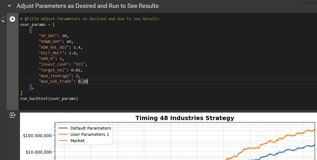
This step involves plotting the cumulative assets under management (AUM) of the portfolio and comparing it with the AUM of the S&P 500 index. To better visualize changes over a wide range of values, we will use a logarithmic scale for the y-axis. The plot will include grid lines, formatted axis labels, and a legend for clarity.
Step 5 Code:
Click to see the Python code
Python
# Ensure 'caldt' is in datetime formatport['caldt'] = pd.to_datetime(port['caldt'])# Set the frequency for plottingfreq = 21# Create the plotfig, ax = plt.subplots(figsize=(10, 6))# Plot the AUMax.plot( pd.concat([port['caldt'].iloc[::freq], port['caldt'].iloc[[-1]]]), pd.concat([port['AUM'].iloc[::freq], port['AUM'].iloc[[-1]]]), linewidth=2, color='k', label='Timing Ind.')# Plot the AUM_SPXax.plot( pd.concat([port['caldt'].iloc[::freq], port['caldt'].iloc[[-1]]]), pd.concat([port['AUM_SPX'].iloc[::freq], port['AUM_SPX'].iloc[[-1]]]), linewidth=1, color='r', label='Market')# Set y-axis to logarithmic scaleax.set_yscale('log')# Set y-axis ticks to double each timeax.yaxis.set_major_locator(LogLocator(base=10.0, numticks=10))ax.yaxis.set_minor_locator(LogLocator(base=10.0, subs=[2, 3, 4, 5], numticks=10))ax.yaxis.set_major_formatter(FuncFormatter(lambdax, pos: "${:,.0f}".format(x)))# Ensure the y-axis labels are visibleax.tick_params(axis='y', which='major', labelsize=10)ax.tick_params(axis='y', which='minor', labelsize=8)# Set x-axis date formatax.xaxis.set_major_formatter(mdates.DateFormatter('%Y'))ax.xaxis.set_major_locator(mdates.YearLocator(10)) # Show x-ticks every 10 years# Add gridax.grid(True, which='both', linestyle='--', linewidth=0.5)# Add legendax.legend(loc='upper left', fontsize=10)# Set titleax.set_title(f'Timing 48 Industries Strategy', fontweight='bold', fontsize=14)# Set x and y limitsax.set_xlim([port['caldt'].iloc[0], port['caldt'].iloc[-1]])# Show the plotplt.tight_layout()plt.show()
Plot:
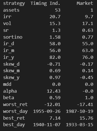
Step 6: Statistical Analysis and Performance Metrics
Overview
This step involves calculating various statistical and performance metrics for the portfolio and market. These metrics include the hit ratio, skewness, Sortino ratio, maximum drawdown, and regression analysis to compute alpha and beta. The results are summarized in a table for easy comparison.